Supply of Resources
The third task of the firm is to obtain resources needed to produce a product. For each resource, a supply curve shows limitations that the firm faces. These supply curves are based on the preferences of sellers and on the actions of other firms that use the resource.
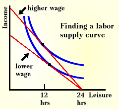
Because a market demand curve can be derived from utility curves and a budget line, it may seem surprising that a supply curve can also be derived from the same procedure. To see that it can, consider the graph below that shows indifference curves for income and leisure. Income is desirable because one can obtain other desirable things with it, and leisure is desirable because it lets one enjoy income.

In the world we live in, greater amounts of income must be purchased with more work--which means less leisure. The tradeoff between leisure and income, shown by the budget line, depends on the wage rate. If the wage rate is $10, options open to an individual include 24 hours of leisure and no income, or 20 hours of leisure and $40 of income, or 10 hours of leisure and $140 of income.
To get a supply curve for labor, one must see what happens if the wage rate changes. Two wage rates are shown in the graph above. At the higher wage rate, the individual wants less leisure (which means he will work more as wages rise), but one could as easily draw indifference curves that show the amount of leisure rising as wages rise (which means he will work less as wages rise). Higher wages have two effects on the leisure-work decision, and these two effects pull in opposite directions. A higher wage rate increases the benefits of working, causing people to substitute work for leisure. This is called the substitution effect and is caused by changes in the slope of the budget line. Higher wages also increase income, and people want more leisure with a higher income. This is called the income effect of a price change and is caused by changes in the distance of the budget line from the origin.
Usually the substitution and income effects reinforce each other, but they pull in opposite directions and almost cancel each other out in the case of labor. Most economists believe that the market supply curve for labor (found by adding up all the supply curves of individuals) is close to a vertical line.
Supply curves for other resources can be obtained in similar ways. The supply curve for capital, for example, depends on decisions of people to consume now or to consume in the future. People who prefer to consume in the future will save and make funds available to finance capital. Their "time preference" determines the shape of indifference curves. The slope of the budget line depends on the interest rates. The budget line tells how much one can get in the future if one sacrifices consumption now.
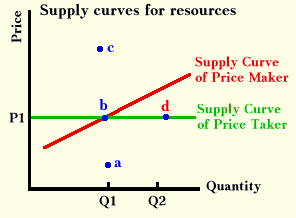
Although the overall market supply curve for labor may be almost vertical, no firm sees this supply curve. Firms hire not general labor, but specific kinds of labor--accountants, electricians, truck driver, etc.--and because people can shift from one occupation to another, the supplies of specific kinds of labor are more elastic than that for labor in general. Also, because there are other many firms buying labor, what one firm does may have little effect on the overall market. If the firm is so small in the market that it can see no effects at all on the wage from its hiring decisions, it is a price taker. If it has some effect on wages, so that when it wants to hire more, it finds that wages rise, the firm is a price maker or what economists usually call a price searcher. The extreme case of a price maker is a monopsonist, the case of only one buyer in the market. The supply curve for a resource that a monopsonist sees is the same as the market supply curve for that specific resource.
The supply curve for a resource is a constraint or boundary on the firm because it shows the minimum that the firm can pay for a level of the resource. If the firm is a price taker in the resource market, it will face a horizontal supply curve such as that in the graph below. This curve indicates that any number can be bought at P1 with no effect on price. There is no way the firm can attain point a even though it might prefer to pay less than P1 because no one will sell at less than P1. Sellers will not sell because we assumed that there were a great many other buyers of the resource who will pay P1. Point c is possible, but a waste of money because the same amount of the resource could be bought for less.

If the firm is one of a few buyers or the only buyer of a resource, it may face a supply curve that slopes upward, making it a price searcher. It can obtain quantity Q1 if it pays P1, but it must pay more than P1 if it wants quantity Q2.
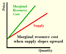
You should have noticed that there are similarities between a supply curve for a resource and a demand curve for output. Both are boundaries, and the curve the firm faces may differ from the market curve. The similarity goes further, because there is a counterpart for marginal revenue called "marginal resource cost" that measures the extra cost to the firm of hiring one more unit of the resource.
When a firm is a price taker, marginal resource cost is the same as the price of the resource. If the firm can hire as many workers as it wants at $10 per hour, then hiring one more hour of labor adds $10 to costs. Marginal resource cost and the supply of labor are both horizontal lines in this case.
When a firm is a price searcher facing an upward-sloping supply curve, the extra cost of hiring another unit of the resource is different from the price of the extra unit. The table below illustrates the reason for this difference. If the firm wants to buy two units, it cannot pay $1.00 and get two. It must be willing to pay $2.00 for each. However, the added cost of the second unit is not $2.00, but $3.00. This can be shown by comparing the total cost of two units and one unit, or $4.00 less $1.00. The added cost of the second unit is not only the two dollars that must be paid for it, but an added dollar for the first one. By the same logic, the added cost of a third unit is $5.00.
|
|
||
|
|
|
Cost |
|
|
|
|
|
|
|
|
|
|
|
|
The marginal resource cost curve lies above an upward-sloping supply curve because of the assumption that the firm can pay only one price. This is often a realistic assumption. If the firm hires two clerks who do exactly the same work, and pays one $4.00 per hour and the other $6.00 per hour, the lower-paid one will be unhappy and may refuse to work for the lower pay. On the other hand, many firms do not publicly disclose what they pay various people, and discourage employees from discussing salaries. To the extent that people are unaware of what others are earning, the firm may be able to pay different prices for the same resource, or in economists' jargon, to price discriminate. Price discrimination will pull down the MRC curve in the graph closer to, or perhaps even onto, the supply curve.

Copyright Robert Schenk